Usage
The core function in VarianceComponentTest.jl is gwasvctest, which wraps the three types of exact tests. The usage for gwasvctest is
gwasvctest(Name = Value)
Where Name is the option name and Value is the value of the corresponding option. Note that it's okay if Value is not provided since every option has a default value.
There are two ways to call gwasvctest
- Open up Julia and type
julia> using VarianceComponentTest
julia> gwasvctest(Name = Value)
- From command line, type
$ julia -E 'using VarianceComponentTest; gwasvctest(Name = Value)'
Background
Consider a standard linear mixed model
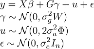
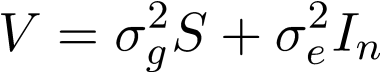
where y is a vector of quantitative phenotype, X is covariate matrix, \beta is a vector of fixed effects, G is genotype matrix for m genetic variants, \gamma is their effects and follows an normal distribution, W is prespecified diagonal weight matrix for the genetic variants, u is vector of random effects included to control familial or structural correlation in the sample, and \epsilon is vector for the error. \Phi is the theoretical kinship matrix or estimated relationship matrix by whole-genome genotypes. \sigma_g^2, \sigma_a^2 and \sigma_e^2 are corresponding variance component parameters from SNP-Set, additive genetic and environmental effects. Therefore,

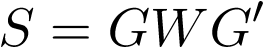
where S is the kernel matrix capturing effects from the SNP set. This software is designed to test
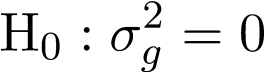
For unrelated sample, \sigma_a^2 is zero, thus the model reduce to
Specify input PLINK files
Option plinkFile indicates the file name (without extension) for the input PLINK files. All three PLINK files have the same file name but different extensions. Make sure the three PLINK files are at the same directory.
If the three PLINK files are plink.bed, plink.bim and plink.fam, then use
gwasvctest(plinkFile = "/PATH/OF/plink")
Replace "/PATH/OF/" with the actual path of PLINK files.
Specify input covariates file
Option covFile indicates the file name for the input covariates file. If the covariates file is covariates.txt, then use
gwasvctest(covFile = "/PATH/OF/covariates.txt")
If option covFile is not specified, the covariates matrix X will be automatically set to a n-by-1 matrix with all elements equal to 1, where n is the number of individuals.
Specify input trait file
Option traitFile indicates the file name for the input trait file. If the trait file is y.txt, then use
gwasvctest(traitFile = "/PATH/OF/y.txt")
If option traitFile is not specified, the response vector y will be set automatically to the phenotypes obtained from the .fam PLINK file.
Specify input annotation file
Option annotationFile indicates the file name for the input annotation file. If the annotation file is annotation.txt, then use
gwasvctest(annotationFile = "/PATH/OF/annotation.txt")
Specify output file
Option outFile indicates the file name for the output file. If the output file name is set to test.out, then use
gwasvctest(outFile = "/PATH/OF/test.out")
Replace "/PATH/OF/" with the path where you want to store the output file. If option outFile is not specified, the output file name will be set to plinkFile-julia.out and it will be stored at the current directory.
Choose testing scheme
ExactVarianceComponentTest.jl provides three types of exact tests: exact likelihood ratio test (eLRT), exact restricted likelihood ratio test (eRLRT) and exact score test (eScore). Option test indicates which testing scheme you want to perform. The usage is
gwasvctest(test = "eLRT"): perform exact likelihood ratio testgwasvctest(test = "eRLRT"): perform exact restricted likelihood ratio testgwasvctest(test = "eScore"): perform exact score test
The default value for option test is eRLRT.
Choose method for computing p-value
Option pvalueComputing indicates which method will be used to obtain the p-value under null hypothesis. The usage is
gwasvctest(pvalueComputing = "MonteCarlo"): use a Monte Carlo method by generating many replicates to obtain the exact null distribution of test statistic and then compute the p-value.gwasvctest(pvalueComputing = "chi2"): use a mixed Chi squared distribution to approximate the null distribution of test statistic and then compute the p-value.
The default value for option pvalueComputing is chi2. The approximation effect of mixed Chi squared distribution has been showed to be good enough, and such approximation will be faster than Monte Carlo method since much less replicates need to be generated. So please use chi2 whenever possible.
Note:
- Option
pvalueComputingis only valid for eLRT and eRLRT, since this software employs the method of inverting characteristics function to compute the p-value for eScore. - In the approximation method, the exact null distributions of eLRT and eRLRT are approximated by a mixture of the form
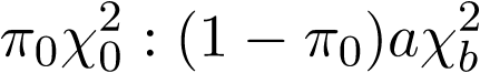
where the point mass \pi_0 at 0, scale parameter a, and the degree of freedom b for the chi-squared distribution need to be determined for each SNP-set. First, estimate \pi_0 by generating B replicates (the number of replicates B is specified by option nNullSimPts), and then estimate a and b using only a small number (300 by default) of replicates.
Choose number of replicates to generate for obtaining null distribution of test statistic and p-value
Option nNullSimPts lets you to decide how many replicates to generate for obtaining null distribution of test statistic and p-value.
- For
pvalueComputing = "MonteCarlo", the more replicates to generate, the more precise the p-value will be (smaller standard error) - For
pvalueComputing = "chi2", the number of replicates only effects the estimate of point mass at 0 for test statistic
nNullSimPts should take positive integer, and the default value is 1,000,000.
Note:
- Option
nNullSimPtsis only valid for eLRT and eRLRT. - For
pvalueComputing = "MonteCarlo", setnNullSimPtsto 10,000 should be sufficient. Otherwise, Monte Carlo method with the default value is too slow.
Choose method for computing kinship matrix
Option kinship indicates how to obtain the kinship matrix. The usage is
gwasvctest(kinship = "none"): Not include kinship matrix in the model, which means there are two terms in the variance structure of response: SNP-set effect and random environmental effect.gwasvctest(kinship = "GRM"): compute kinship matrix by genetic relationship matrix (GRM). The algorithm is provided in section 2.3 by Zhou et al.gwasvctest(kinship = "MoM"): compute kinship matrix by method of moments (MoM). The algorithm is provided in section 2.3 by Zhou et al.gwasvctest(kinship = "theoretical"): compute kinship matrix theoretically.gwasvctest(kinship = "FILE"): replace FILE with the file name in which store your own pre-calculated kinship matrix.
The default value for option kinship is GRM.
Choose weights for SNP-set effect
Option snpWtType indicates the diagonal elements for the diagonal weight matrix W for each SNP-set. The usage is
gwasvctest(snpWtType = ""): Constant weights, i.e., set all weights to 1gwasvctest(snpWtType = "beta"): Beta weights, i.e., set the weights by a beta distribution Beta(1, 25) evaluated at MAF for each SNPgwasvctest(snpWtType = "invvar"): Inverse variance weights, i.e., set the weights by inverse variance 1/sqrt(MAF*(1-MAF))
The default value for option snpWtType is empty.
Choose method for computing kernel matrix
Option kernel indicates how to obtain kernel matrix S. The usage is
gwasvctest(kernel = "GRM"): compute kernel matrix S by genetic relationship matrix (GRM), i.e. S=GG', where G is genotype matrix.gwasvctest(kernel = "IBS1"): compute kernel matrix by IBS1.gwasvctest(kernel = "IBS2"): compute kernel matrix by IBS2.gwasvctest(kernel = "IBS3"): compute kernel matrix by IBS3.
The default value for option kernel is GRM.
The standard IBS kernel values are showed in following tables
Table 1: IBS1 Kernel Values || Table 2: IBS2 Kernel Values || Table 3: IBS3 Kernel Values
| i/j | 1/1 | 1/2 | 2/2 | i/j | 1/1 | 1/2 | 2/2 | i/j | 1/1 | 1/2 | 2/2 | ||||
|---|---|---|---|---|---|---|---|---|---|---|---|---|---|---|---|
| 1/1 | 1 | 0.5 | 0 | 1/1 | 0.5 | 0.5 | 0 | 1/1 | 1 | 0.5 | 0 | ||||
| 1/2 | 0.5 | 0.5 | 0.5 | 1/2 | 0.5 | 1 | 0.5 | 1/2 | 0.5 | 1 | 0.5 | ||||
| 2/2 | 0 | 0.5 | 1 | 2/2 | 0 | 0.5 | 0.5 | 2/2 | 0 | 0.5 | 1 |
where i and j indicate two individuals. The IBS kernels are determined by
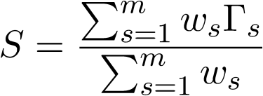
where w's are the weights for the m SNPs, \Gamma_s is the covariance matrix depending only on the genotypes at SNP s. The values of \Gamma_s are read from the above three tables.
Determine the rank used to approximate the kinship matrix
In our algorithm, we do a low rank approximation of kinship matrix to reduce the multiple variances components testing problem to two variance components problem. However, there is a trade-off for choosing the rank for approximating: if the rank is high, then a better approximation can be obtained, but a high rank will lead to a small signal-to-noise ratio, which will decrease the power of test.
Option infLambda provides a way to control such trade-off. Theoretically, infLambda can take any real value. If infLambda takes non positive value, then the algorithm will take the highest possible approximating rank. If infLambda takes a positive value, the algorithm will take a smaller approximating rank, and the larger the value is, the smaller the approximating rank will be. The default value is 0.
For example, want to take the highest rank, then
gwasvctest(infLambda = 0.0)
Note: If you are analyzing unrelated data, you can ignore option infLambda since the kinship matrix will not be included in the model in unrelated case.
Determine the group size for each SNP set
Option windowSize determines the group size of a SNP set for which you want to test. It can only take positive integer. The default value is 50.
For example, want to set the group size to 60, then
gwasvctest(windowSize = 60)
Note that if annotation file is provided, the group size will be determined automatically, so you don't need to specify windowSize in that case.
Parallelization
Modern computer has multiple cores usually. So you can take advantage of the parallel computing mode provided by this package
julia> addprocs(n)
julia> using VarianceComponentTest
julia> gwasvctest(Name = Value)
where n is the number of working processes which are employed to perform the computations. Usually, n is the number of cores your machine has.
You can also active the parallel mode from command line
$ julia -p n -E 'using VarianceComponentTest; gwasvctest(Name = Value)'
where n has the same meaning as above.
A concrete example is provided at the Example part.
Note: In Linux system, you can use the following shell command to count the number of cores on your CPU
$ cat /proc/cpuinfo | grep processor | wc -l